Nucleation¶

MICRESS® offers a number of submodels to simulate nucleation under assumption of different material and process specific conditions. Note that nucleation conditions have to be specified for each phase, individually. Without a given nucleation condition, a new phase will not appear. Nucleation conditions are always defined with respect to a certain reference phase and with respect to a certain nucleation position, e.g. the bulk of the phase or the interface to another phase. Nucleation will occur when the local undercooling evaluated with respect to the reference phase exceeds the critical undercooling required for nucleation. The critical undercooling can either be defined by the user as a fixed value or evaluated based on a specific criterion, e.g. for heterogeneous nucleation on inoculant particles.

Activation of nucleation¶

The keyword nucleation activates nucleation input. In the following, the number of different nuclei types (here referred to as 'seed types') is requested.

...
# Nucleation
# ==========
# Enable further nucleation?
# Options:  nucleation   nucleation_symm   no_nucleation
nucleation
#
# Number of types of seeds?
1
...

Define seed types¶

Seed position
Seed model
seed growth model
Shield effect
Other settings, e.g. nucleation range, time check interval

Example 1¶

One seed type in the bulk

...
# Type of 'position' of the seeds?
# Options:   bulk  interface  triple  quadruple  front  [restrictive]  [region]
bulk
# Phase of new grains (integer) [unresolved|add_to_grain|split_from_grain]?
2
# Reference phase (integer) [min. and max. fraction (real)]?
1
# Which nucleation model shall be used?
# Options:    seed_undercooling    seed_density  [ lognormal_1 | lognormal_2 ]
seed_undercooling
# Grain radius [micrometers]?
0.00000
# Choice of growth mode:
# Options:   stabilisation analytical_curvature
stabilisation
# min. undercooling [K] (>0)?
15.000
# Shield effect:
# Shield time type [shield phase/group]?
# Options:  constant   automatic   [shield phase or group number]
constant
# Shield time [s] ?
20.000
# Shield distance [micrometers] ?
7.500000000000
# Nucleation range
# min. nucleation temperature [K]
0.000000000000
# max. nucleation temperature [K]
1200.000000000
# Time between checks for nucleation? [s]
# Options:  constant   from_file   automatic
constant
# Time interval [s]
0.25000
# Check distance [micrometers]
7.500000000000
# Maximum number of nuclei (-1 for unlimited)
#   [Maximum number of simultaneous nucleations (default -1 for unlimited)]?
500
# Shall random noise be applied?
# Options:     nucleation_noise   no_nucleation_noise
no_nucleation_noise
# Random number seed for positions [orientations, noise]?  (integer(s))
77777
# Shall metastable small seeds be killed?
# Options:     kill_metastable      no_kill_metastable
no_kill_metastable
# Verbose mode
# Options: verbose  no_verbose
no_verbose
...

Seed position¶

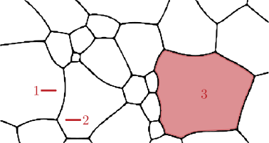
Seeds can either be placed in the bulk, at interfaces, at triple or quadruple junctions or at a certain distance to a given phase (front), as illustrated in Figure 1. Note that by default, bulk includes interfaces, interface includes triple junctions, triple junctions includes quadruple junction, and those all other high-order junctions. The optional parameter 'restrictive' allows to address pure 'bulk' without interfaces, or pure interface without triple junctions and so on. The optional parameter region allows to restrict nucleation to a specific region of the simulation domain. The minimum and maximum coordinates are requested (in $\rm{\mu m}$ ) for each direction. To trigger nucleation at a predefined point, equal minimum and maximum values may be selected. In case of front, the nuclei are placed within the reference phase, but at a certain distance to the substrate phase. This distance is specified by the user in a separate line.

Figure 1¶

Illustration of seed position options

$1$ : interface. $2$ : triple junction. $3$ : bulk

For each seed type, the phase of the seed (nuclei) as well as the reference phase must be defined. Note that nuclei can appear only at places where the reference phase is present. In the case of concentration coupling, the driving force for nucleation is calculated as function of the local composition of this phase. In solidification simulations, the reference phase is typically the liquid phase.

In case of nucleation on interfaces or junctions, specification of an additional substrate phase is requested, see Example 2. Nucleation will only occur at interfaces where the substrate phase is present. If an additional, optional second substrate phase is specified, nucleation will only occur at interfaces or junctions where both phases coexist. Both substrate phases may be defined equal to model nucleation on grain boundaries, only. The curvature of the first substrate determines the curvature contribution to the nucleation undercooling. This curvature contribution is disregarded if the substrate phase is identical to the reference phase. In the case of front, the substrate phase determines in front of which phase nucleation shall happen.

In the same line with the phase number of the new grain, optional models can be specified, namely unresolved, add_to_grain or split_from_grain.

The option unresolved invokes a model in which fine eutectic or eutectoid phases are treated as a continuous phase mixture (see chapter Diffuse Phase Model for unresolved eutectic-or-eutectoid regions).

The option add_to_grain allows nucleation of a grain which already exists in a second place, as shown in Example 2. As the properties of the grain will be overwritten by those specified in the nucleation parameters, the option add_to_grain allows also changing properties of an existing grain. The suboptions grain_number, phase_number, parent_grain or new_set must be chosen in the next line. For details see chapter Advanced Grain Manipulation.

The purpose of the option split_from_grain is to transform a disconnected part of a grain to a new grain. The new grain number and the grain properties specified in the nucleation parameters apply only to the part which is split off. The suboptions grain_numberor parent_grain as well as an optional input of the maximum size must be chosen in the next line. For details see chapter Advanced Grain Manipulation.

Furthermore, the minimal and maximal fraction of the reference phase where new nuclei are allowed to appear can be optionally specified in the same line with the reference phase number. This allows the user, for example, to place new seeds at the outer part of a solid-liquid interface which increases their chances to grow before getting overgrown by the advancing solidification.

Example 2¶

Position type interface and advanced option add_to_grain

...
# Type of 'position' of the seeds?
# Options:   bulk  interface  triple  quadruple  front  [restrictive]  [region]
interface
# Phase of new grains (integer) [unresolved|add_to_grain|split_from_grain]?
2 add_to_grain
# Which grain number the new grains shall be added to?
# # Options:   grain_number (number)  phase_number (number)  parent_grain   new_set
grain_number 0
# Reference phase (integer) [min. and max. fraction (real)]?
0 0.95 1.
# Substrat phase [2nd phase in interface]?
1 3
...

Seed model¶

In case of nucleation in bulk, MICRESS® allows the user to choose between the standard 'seed undercooling' and the so-called 'seed density' model, which models heterogeneous nucleation on virtual particles randomly distributed in the melt.

`seed_undercooling` model¶

Example 3¶

Further nucleation using the seed undercooling model

...
# Which nucleation model shall be used?
# Options:    seed_undercooling    seed_density  [lognormal_1 | lognormal_2]
seed_undercooling
# Grain radius [micrometers]?
0.0
...

`seed_density` model¶

Figure 2¶

Seed density classes

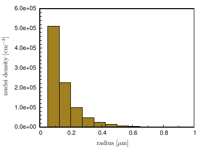
Using the given density, explicit positions of the potential nucleation sites are determined. The radii (and thus the local critical undercooling for nucleation on each particle) are distributed evenly according to the radius range of each seed class. Inside each class, a random radius distribution is assumed. The radius range corresponds to the radius difference to the next specified class. The finally created numbers and radius ranges for each class can be found in the .log-file.

In MICRESS®, the seed density distribution can be either defined manually by using a table form, or be generated automatically by defining a lognormal density function. In the case of table form (see Example 4), the seed classes must be specified starting with the highest radius values. At least two classes should be specified otherwise the automatically assumed radius range may lead to unexpected results.

Optionally, an additional clustering of the randomly distributed seeds can be obtained. This is done by specifying an additional cluster radius and a cluster density in the same line for each class (i.e. four real numbers in each line). The option can be helpful if experimentally a clustering of primary precipitates is observed like in some hypereutectic Al-Si alloys.

Example 4¶

Bulk nucleation using the seed density model

...
# Which nucleation model shall be used?
# Options:    seed_undercooling    seed_density [lognormal_1 | lognormal_2]
seed_density
# Number of seed classes?
10
# Specify radius [micrometers] and seed density [cm**-3] for class  1
0.45 1000
# Specify radius [micrometers] and seed density [cm**-3] for class  2
0.3 2000
# Specify radius [micrometers] and seed density [cm**-3] for class  3
0.25 5000
# Specify radius [micrometers] and seed density [cm**-3] for class  4
0.18 10000
# Specify radius [micrometers] and seed density [cm**-3] for class  5
0.15 20000
# Specify radius [micrometers] and seed density [cm**-3] for class  6
0.12 50000
# Specify radius [micrometers] and seed density [cm**-3] for class  7
0.10 90000
# Specify radius [micrometers] and seed density [cm**-3] for class  8
0.08 140000
# Specify radius [micrometers] and seed density [cm**-3] for class  9
0.07 250000
# Specify radius [micrometers] and seed density [cm**-3] for class 10
0.06 500000
# Determination of nuclei orientations?
...

For generating seed classes using lognormal function, either lognormal_1 or lognormal_2 option should be added next to the option seed_density. In the case of lognormal_1 (see Example 5), the user is required to give the median radius $[\rm \mu m]$ and the standard deviation to define the lognormal density function. By lognormal_2 (see Example 6), the lognormal distribution function is determined by the most frequent radius $[\rm \mu m]$ and an additional specific radius $[\rm \mu m]$ . Here, the specific radius indicates a radius by a specific cumulative distribution function(CDF) value. The user is also allowed to specify the CDF value. By default, the CDF value is set to be 0.99 (or 99%), which corresponds to the maximal radius in the system. In Example 6), the value CDF=0.5 is given, then the specific radius is equivalent to the median radius. More details please refer to the section Lognormal distribution.

Example 5¶

seed density model with option lognormal_1

...
# Which nucleation model shall be used?
# Options:    seed_undercooling   seed_density [lognormal_1 | lognormal_2]
seed_density lognormal_1
# Median radius in micrometer?
0.05000
# Standard deviation ?
1.00000
...

Example 6¶

seed density model with option lognormal_2

...
# Which nucleation model shall be used?
# Options:    seed_undercooling    seed_density [lognormal_1 | lognormal_2]
seed_density lognormal_2
# Most frequent radius in micrometer?
0.02000
# Specific radius in micrometer [<CDF value> (Default: 0.99)]
0.05632 0.5
...

After the determination of the lognormal density function, some parameters are needed for the generation of the seed classes: the number of classes, the total particle density $[\rm cm^{-3}]$ in the simulation region, and a range of radius in which the nucleation most probably takes place.

...
# Generate seed density classes:
# Number of seed classes?
10
# Total seed density in cm**-3?
0.20000E+07
# Range of considered seed radius in micrometer?
# <radiusMin>  <radiusMax>
0.05500   0.52500
...

Small seed treatment¶

For defining the grain growth model, the user should choose either stabilisation or analytical_curvature, and define the minimal undercooling. Details about how to choose them is described in section Microstructure.

...
# Grain radius [micrometers]?
0.0000
# Choice of growth mode:
# Options:   stabilisation analytical_curvature
stabilisation
# min. undercooling [K] (>0)?
10.000
...

If the new phase is not isotropic (see Phases/anisotropy), the orientation of the new grains has to be specified. A random distribution, a fix value, an orientation range or a parent relation, i.e. a relative orientation to the grain of the local substrate phase, can be chosen. The option parent_relation applies only to nucleation at interfaces or junctions. For the option fix, the rotation angle should be given according to which relative rotation option has been chosen for the nuclei phase, see Phases/Crystallographic orientation.

...
# Determination of nuclei orientations?
# Options:   random    randomZ   fix     range    parent_relation
fix
# Rotation angle? [Degree]
38.000
...

Shield effect¶

Other settings¶

If in section Phases, categorize and anisotropic have been chosen for the nuclei phase, the user has to decide whether for this seed type categorization of the orientation values to orientation categories shall be performed. This is important, if different grains shall be assigned to the same grain number during run-time, because this is only possible if all grain properties including orientations of the grains are identical (see Phases). After the keyword categorize, the number of orientation categories can be specified, default is 36 (corresponding to 10° difference between the orientation categories in 2D).

...
# Shall categorization be applied to this seed type?
# Options:    categorize  {Number}   no_categorize
categorize 36
...

For RX nucleation, the user has to specify also a minimal and maximal energy or alternatively dislocation density of the nuclei. Classically, these energies are zero. In this case, RX starts directly. If these energies differ from zero, RX simulation starts later and an initial microstructure can be built up for example in the case of RX simulation after a solidification analysis. When specifying dislocation densities, their value must be very small and significantly lower than the specified dislocation threshold.

Further, MICRESS® requests a minimum and a maximum nucleation temperature for the actual seed type. A minimum and maximum temperature should be chosen around the temperature where nucleation is expected. The parameters primarily help to minimize unnecessary nucleation checks and thus to improve performance. In some cases with TQ coupling, checking nucleation too far from the temperature where the new phase gets stable can cause numerical problems. Then, proper values have to be found, depending on the system. In a first trial, it is wise not to restrict the nucleation range.

The time between checks for nucleation determines the frequency of nucleation checking. If chosen too high, insufficient seeding may occur in spite of high local undercooling. If chosen too small, an unnecessarily high numerical effort and a corresponding performance loss can be the consequence. Note that in case of TQ coupling, each check for nucleation requires time-consuming calls to the TQ interface for each checked position. A possible performance loss can be monitored using the .TabP or .TabTQ output. Time-dependent checking frequencies can be specified by input from file.

The 'automatic' mode allows to specify a temperature delta. Each time, the temperature has decreased or increased by this temperature, a check for nucleation will be done.

Nucleation checks are performed for all cells in a bulk or interface region. The computational expensive check for undercooling will be done if other conditions are met, e.g. phases exists, no previous grain shields, etc. Nevertheless, a lot of cells of interest can be left. The 'check distance' parameter to reduce this workload further. If a cell with a high enough undercooling is found, no cells in the check distance neighbourhood will be checked.

The number of nuclei of a seed type can be limited. Optionally, the number of simultaneous nucleation events of a seed type can also be limited. A list of possible seeds is created and ordered with respect to the undercooling or driving force for each nucleus. If the maximum number is exceeded, the less favourable seeds are discarded.Usually, it is recommended to start with an unlimited number (-1 to set it).

...
# Nucleation range
# min. nucleation temperature [K]
0.00
# max. nucleation temperature [K]
820.00
# Time between checks for nucleation? [s]
# Options:  constant   from_file   automatic
automatic
# Bottom Temperature change between checks for nucleation [K]
0.10
# Check distance [micrometers]
10.00
# Maximum number of nuclei (-1 for unlimited)
#   [Maximum number of simultaneous nucleations (default -1 for unlimited)]?
-1

Noise can be added to the nucleation undercooling. In that case, the amplitude for the noise level and a seed for the random number generator will be asked later (see below).

The noise is applied as

$\Delta G \leftarrow [1+k({\rm random} -0.5)]\Delta G$

where $k$ is user defined noise amplitude, $0 \le {\rm random} \le 1$ is the value of the random number generator and $\Delta G$ is the nucleation driving force.

...
# Shall random noise be applied?
# Options:     nucleation_noise   no_nucleation_noise
nucleation_noise
# Factor for random noise?
# (applied as DeltaT -> (1+Factor*(RAND-1/2))*Delta
0.1
...

Each seed type, uses its own sequences of random numbers. Different sequences are used to determine nuclei's positions, orientation and noise to apply. The integer number to initialize the random number generator for the position sequence is mandatory. The other ones are optional and will be set to a default if not given. As the default is different for each type (depending on the type index), the sequences will differ.

In some cases, "stabilised" small grains can erroneously reach a metastable state at which they stop growing, but also do not vanish because their stabilisation implies a reduced curvature. By enabling the flag kill_metastable, the stabilisation of small grains is removed after their shield time has elapsed. This makes sure that "metastable grains" can vanish correctly. The option kill_metastable is also relevant in case of categorization, because after "killing", small stabilized grains are considered as "big" and such can be assigned to a common grain number.

Important: The kill_metastable flag is only relevant for small grains which use the stabilisation model.

Finally, a verbose screen output for nucleation of this type can be enabled. This additional output provides information on the number of potential and successful nucleation events. This option is very helpful to find out why a given set of nucleation parameters is not leading to the desired result, but is not recommended to be used during standard simulation.